
2d-decision-integrator
A spiking model of perceptual decision making built from a single two-dimensional integrator. MT drives a noisy 2D LIP population whose recurrent feedback accumulates evidence in any direction at once; an output ensemble starts spiking once the integrator crosses an intercept threshold.
Description
This is the standalone example from chapter 8 of How to Build a Brain (Eliasmith, 2013), distributed with nengo-gui as 2D_decision_integrator.py.
The intuition the chapter develops: rather than running one integrator per task dimension, you can fold them all into a single multi-dimensional integrator and let the geometry of the input pick the direction. Here that's a 2D LIP ensemble — its recurrent self-connection makes it a leaky integrator, and the input from MT pushes it in whichever direction the stimulus favours. Both MT and LIP carry injected white noise so the trial-to-trial trajectories are stochastic, which is the point — the model accumulates evidence under noise, not a clean signal.
The default inputs are (input1, input2) = (-0.5, 0.5); sliders are wired up in the .cfg so you can sweep them live in NengoGUI and watch LIP drift in the new direction.
Four ensembles, in flow order:
ens_inp— 2D representation of the two scalarinput1/input2nodesMT— 2D ensemble with white noise (motion-area analogue, just a noisy relay here)LIP— 2D ensemble with recurrent self-connection and white noise (the integrator)ens_out— 2D output ensemble with high intercepts (≥0.3), so it only spikes when LIP crosses threshold
The MT→LIP connection has a small transform=0.1 and a 100 ms synapse — the same time-scale as the LIP recurrence — so the integrator approximates a leaky accumulator with τ ≈ 100 ms.
Run it
In NengoGUI (the intended way to view it):
pip install nengo-gui
nengo 2d_decision_integrator.py
Or just at the command line:
python 2d_decision_integrator.py
To see the threshold-crossing effect, the .cfg already wires up a Raster plot of ens_out: spikes are sparse early in a trial, then dense once LIP has accumulated enough evidence to push past the output ensemble's intercept threshold.
How it works
The 2D LIP recurrence with synapse=0.1 and identity transform implements dx/dt ≈ (input − x)/τ with τ = 0.1 s, i.e. a leaky integrator in two dimensions. With noise injected directly into MT and LIP, the state diffuses in the integrator plane, biased in the direction of the input. Because LIP is a single 2D ensemble (not two scalar ensembles wired in parallel), one population represents the full 2D state with shared neurons — neurally cheaper, and the chapter's main point.
ens_out has its intercepts shifted to Uniform(0.3, 1): every neuron in it has a high firing threshold, so the output is approximately silent until LIP's magnitude exceeds ~0.3 in some direction. That's what produces the "decision" — a sudden ramp of output firing once enough evidence has accumulated.
The seed=11 on the network makes the noise reproducible across runs.
Citation
@book{eliasmith2013htb,
  author    = {Eliasmith, Chris},
  title     = {How to Build a Brain: A Neural Architecture for Biological Cognition},
  publisher = {Oxford University Press},
  year      = {2013}
}
License
GPLv2 (see LICENSE).
Figures
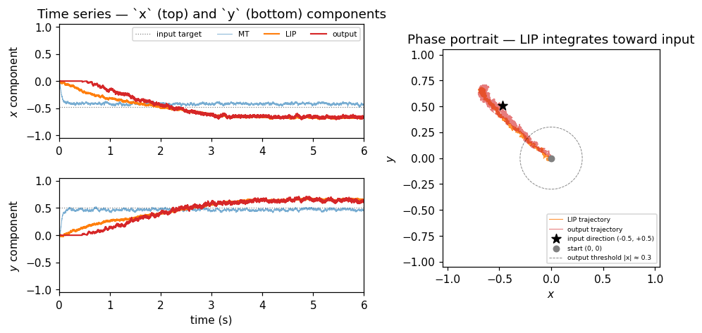
6 seconds of the 2-D decision integrator, produced by running 2d_decision_integrator.py directly.
The network is presented with a constant 2-D input (-0.5, +0.5) corrupted by independent white-noise injections on the MT, LIP, and output ensembles, modelling the noisy evidence stream a perceptual decision-making circuit would receive.
Left — time series. The x (top) and y (bottom) components of the decoded state in MT (light blue), LIP (orange), and the output ensemble (red), with the input target as a dotted gray line. MT jumps to the input value within milliseconds and then jitters around it; LIP integrates over the next ~2 seconds and starts to track the input value; output follows LIP after a further delay because its intercepts are clamped to ≥ 0.3, so it only fires once LIP's magnitude has crossed that threshold.
Right — phase portrait. LIP's 2-D trajectory (orange) wanders from the origin (gray dot) toward the input direction (black star at (−0.5, +0.5)). The output trajectory (red) covers the same path but only after LIP escapes the dashed threshold circle. The wandering after t ≈ 3 s is the integrator amplifying the injected ensemble noise.