
controlled-oscillator
A 2D oscillator whose angular speed is gated by a third recurrent dimension — and that gate, in turn, is driven by a separate input ensemble. A clean demonstration of one neural population controlling the dynamic regime of another.
Description
This is the controlled-oscillator pattern from the CNRG tutorial series. The differential equations are the same as a plain oscillator — a 2D circle in state space — but the angular speed s is itself a dimension of the same ensemble:
dx0/dt = -x1 · s + x0 · (r - x0² - x1²)
dx1/dt =  x0 · s + x1 · (r - x0² - x1²)
A separate speed ensemble feeds the third dimension x[2]. Slide the input slider in NengoGUI and watch the oscillator speed up or stop.
Run it
In NengoGUI:
pip install nengo-gui
nengo controlled_oscillator.py
License
GPLv2 (see LICENSE).
Figures
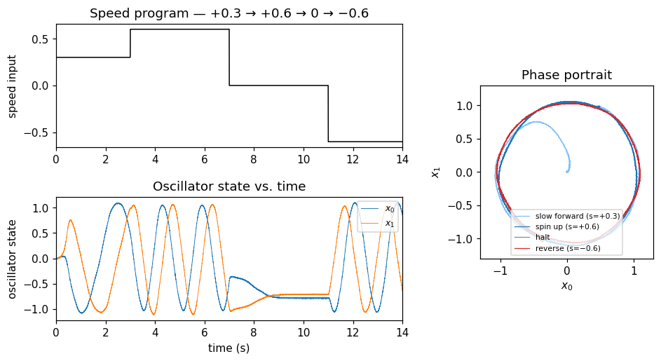
14 seconds of the controlled oscillator driven through a four-segment speed program, produced by running controlled_oscillator.py directly.
Top-left — speed program. The stim_speed input held at four levels: +0.3 (slow forward), +0.6 (faster forward), 0 (halt), −0.6 (reverse). In NengoGUI this input is a slider; here it's stepped programmatically to produce the figure.
Bottom-left — oscillator state vs. time. The 2-D oscillator state (x₀, x₁) over the run. With s = +0.3 the network rotates around the limit cycle at a low rate; with s = +0.6 it rotates roughly twice as fast. When the speed is reset to zero the state freezes at whatever phase it had reached. Flipping the sign reverses the direction of rotation.
Right — phase portrait. The trajectory in the (x₀, x₁) plane, coloured by speed regime. The transient from the origin out to the unit circle (light blue) is the limit-cycle attraction during the initial s = +0.3 segment; the dark-blue and red curves are the faster forward and reverse rotation phases.