
lmu
A drop-in Legendre Memory Unit subnetwork for Nengo — compress a sliding window of an input signal into a low-dimensional Legendre representation, then read off any function of the window (linear or nonlinear) from the state.
Description
The LMU, introduced by Voelker, Kajić & Eliasmith (NeurIPS 2019), maintains a high-fidelity, low-dimensional state vector x(t) ∈ R^q that parameterises the last theta seconds of a scalar input in the Legendre polynomial basis:
u(t − s) ≈ Σₖ xₖ(t) · Pₖ(2 s / theta − 1) for s ∈ [0, theta]
This means:
- Any linear functional of the windowed input (delay, derivative, moving average, low-pass...) has a fixed linear readout from
x(t). No learning is required — just multiply by the right transform. - Any nonlinear functional (RMS, variance, peak, threshold-crossing rate, a learned classifier output, ...) can be computed by routing
x(t)into a Nengo ensemble whose decoders are trained (e.g. by PES) onto the target signal.
This submission ships the LMU as a clean nengo.Network subclass that can be dropped into any model. The headline example (examples/example_usage.py) demonstrates the nonlinear-readout pattern by learning the windowed RMS of a band-limited input — the simplest function that's genuinely nonlinear in the window. The same network shape learns any other windowed nonlinearity by swapping the target signal; the principle is general, and the same machinery extends to classification, regression on stored templates, learned spectral features, or anything else you can compute from a window of the input.
What changed since v0.1.0
- The LMU was refactored from a top-level NengoGUI script into a reusable
LMU(nengo.Network)class undersrc/lmu/. - The headline example is now a windowed-RMS learning task, which is properly nonlinear in the windowed input (a fixed delay is technically a linear functional, and could be computed with a fixed decode).
- The v0.1.0 delay-learning task is preserved as
examples/delay_task.pyfor reference and direct comparison. - The cell-by-cell notebook walkthrough is now at
examples/lmu.ipynb.
Installation
python -m venv .venv
source .venv/bin/activate          # Windows: .venv\Scripts\activate
pip install -r requirements.txt
Usage
import nengo
from lmu import LMU

with nengo.Network() as model:
    stim = nengo.Node(lambda t: ...)                  # any scalar input

    # The LMU subnetwork — compresses the last theta seconds of `stim`
    # into an `order`-dimensional state vector.
    lmu = LMU(theta=1.0, order=8, dt=0.001)
    nengo.Connection(stim, lmu.input, synapse=None)

    # Read off some function of the window. For a nonlinear function,
    # plug the LMU state into a Nengo ensemble and train PES against
    # your target signal (see examples/example_usage.py).
    ens = nengo.Ensemble(800, dimensions=8)
    nengo.Connection(lmu.state, ens, synapse=None)

    out = nengo.Node(size_in=1)
    nengo.Connection(
        ens, out, function=lambda x: 0.0,
        learning_rule_type=nengo.PES(1e-3),
    )
For a complete worked example see examples/example_usage.py (windowed RMS) and examples/delay_task.py (fixed delay, ported from v0.1.0). The companion notebook examples/lmu.ipynb walks through the math.
How it works
The LMU is the analytical impulse-response solution to "best low-rank LTI approximation of a sliding window of input." The continuous-time state-space matrices A ∈ R^(q×q) and B ∈ R^(q×1) are derived from Padé approximants of the pure-delay transfer function projected onto the Legendre basis (see Voelker et al. 2019, Sec. 2). Discretising at the simulator's dt (zero-order hold) gives the matrices used here, and the recurrent connection state → state with transform = A_d and synapse = 0 realises the discrete-time LTI system natively in Nengo.
The state output of the network is just an order-dimensional vector; the Legendre-basis interpretation matters when you want to decode a function of the window, but for downstream learning you can simply treat state as a fixed-dimensional embedding of the last theta seconds of input and train anything you like off it.
Citation
@inproceedings{voelker2019lmu,
  author    = {Voelker, Aaron R. and Kaji{\'c}, Ivana and Eliasmith, Chris},
  title     = {Legendre Memory Units: Continuous-time representation in recurrent neural networks},
  booktitle = {Advances in Neural Information Processing Systems 32 (NeurIPS 2019)},
  year      = {2019},
}
License
GPLv2 (see LICENSE). Matches Nengo's license.
Figures
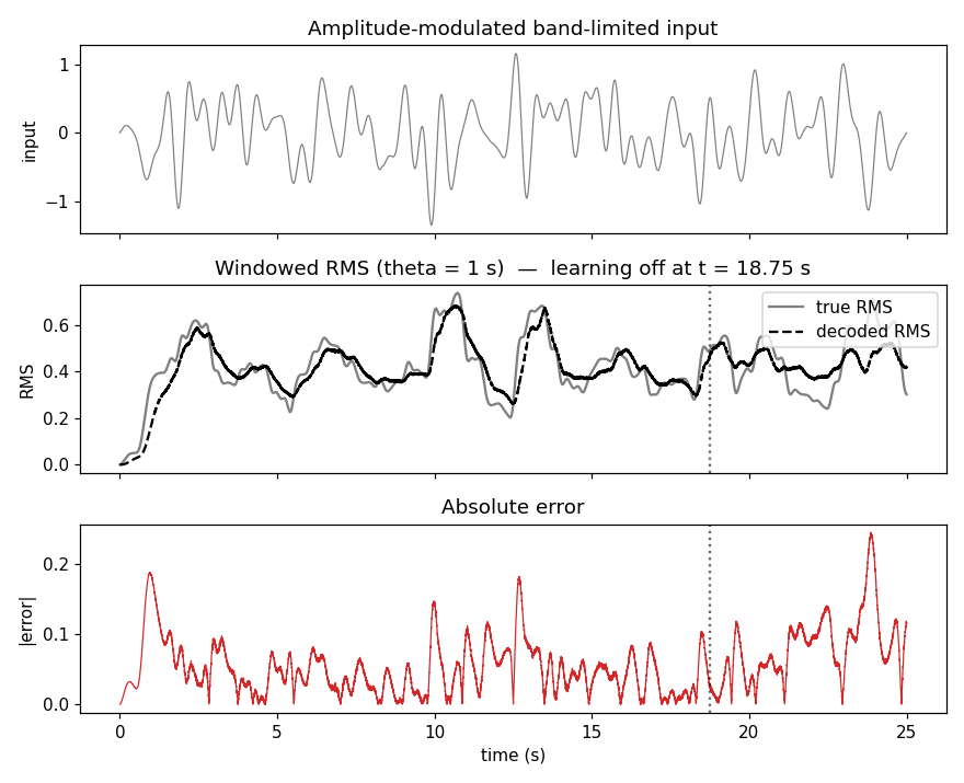
Headline output of examples/example_usage.py: a downstream spiking ensemble reading the LMU state and trained with PES to compute the windowed RMS (root-mean-square over the last theta = 1 s) of the LMU's scalar input.
Top — input. A band-limited (≤ 2 Hz) white-noise carrier multiplied by a slow ( ≤ 0.2 Hz) envelope, so the input's local amplitude varies meaningfully over the 25 s run and the windowed RMS target has visible structure rather than being roughly constant.
Middle — windowed RMS. True windowed RMS (gray) overlaid with the spiking-ensemble decode (dashed black). The vertical dotted line marks where the PES learning rule is switched off (75 % of the way through the run). The decoded RMS stays close to the true target both during training and after learning is shut off — the downstream ensemble has learned a nonlinear function of the LMU state.
Bottom — absolute error. Per-timestep |true − decoded|. Mean over the final 1 s ≈ 0.09; the largest excursions correspond to fast envelope transitions where the network has to update its estimate quickly.
The same network architecture (LMU → spiking ensemble → PES-trained decoder) can learn any nonlinear function of the windowed input (e.g., variance, peak amplitude, threshold-crossing rate, a classifier) by swapping the target signal that PES is given.