
lorenz
A spiking implementation of the Lorenz chaotic attractor. The canonical demonstration that spiking ensembles can sustain non-trivial nonlinear dynamics — and visually striking when watched in NengoGUI.
Description
A single 3D Nengo ensemble (600 spiking neurons) implements the Lorenz system with parameters σ=10, β=8/3, ρ=28. Recurrent connections compute the right-hand side of the differential equations, producing the characteristic two-lobe "butterfly" trajectory. The equations are slightly transformed from the standard Lorenz form to centre the attractor on the origin — see Eliasmith (2005) for the derivation.
This is a GUI-first submission: the canonical artifact is the NengoGUI-runnable script. Open it in NengoGUI to watch the spiking neurons trace the attractor in real time across three XY plots.
Run it
We recommend a fresh virtual environment to avoid Nengo/NumPy version conflicts with your global Python install:
python -m venv .venv
source .venv/bin/activate          # Windows: .venv\Scripts\activate
pip install -r requirements.txt
In NengoGUI:
pip install nengo-gui
nengo lorenz.py
Headless (e.g. to dump a trajectory for offline analysis):
python -c "import nengo; \
from importlib import import_module; \
m = __import__('lorenz').model; \
sim = nengo.Simulator(m); sim.run(5); print(sim.data)"
How it works
The Lorenz system, in the slightly recentered form used here:
dx0/dt = -σ·x0 + σ·x1
dx1/dt = -x0·x2 - x1
dx2/dt =  x0·x1 - β·(x2 + ρ) - ρ
A single 3D ensemble x (radius 30, 600 spiking neurons) feeds back into itself through a lorenz(x) function that computes the synapse-corrected update:
out[i] = synapse · dx_i/dt + x[i]
with synapse = 0.1. The ensemble's recurrent connection (with that same synaptic time constant) closes the loop. The result: a stable chaotic attractor implemented entirely in spikes.
Citation
@article{eliasmith2005attractor,
  author  = {Eliasmith, Chris},
  title   = {A unified approach to building and controlling spiking attractor networks},
  journal = {Neural Computation},
  volume  = {7},
  number  = {6},
  pages   = {1276--1314},
  year    = {2005}
}
License
GPLv2 (see LICENSE).
Figures
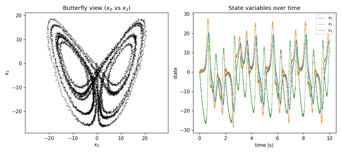
10 seconds of the spiking Lorenz attractor's trajectory, produced by running lorenz.py directly.
Left — "butterfly" view. A 2-D projection of the 3-D state onto (x₀, x₂), the canonical view from Eliasmith (2005). The two lobes are the attractor's signature: the trajectory winds around one lobe for a while, then unpredictably switches to the other.
Right — state variables over time. All three dimensions (x₀, x₁, x₂) traced through the 10-second window, showing the chaotic but bounded oscillations the 600-neuron 3-D ensemble produces by recurrent connection through the Lorenz vector field.